Bézier Curves and De Casteljau's Algorithm
Bresenham's line algorithm and the midpoint circle algorithm draw shapes that are defined by a formula: a line, a circle. Most curves in practice are not like that. The outline of a letter in a font, a path in an SVG file, or a curve in a drawing program is a shape someone designed by hand, and the most common way to describe such shapes is the Bézier curve: a handful of control points that pull the curve into shape without the curve necessarily passing through them.
Bézier curves are named after Pierre Bézier, who popularized them for car body design at Renault in the 1960s. Paul de Casteljau had developed the same curves a few years earlier at Citroën, and the algorithm that bears his name is still the most intuitive way to compute them.
The idea
Everything starts with linear interpolation: given two points A and
B and a number t between 0 and 1, the point lerp(A, B, t) lies on
the straight line from A to B, a fraction t of the way along. At
t = 0 it is A, at t = 1 it is B, at t = 0.5 it is exactly in the
middle.
De Casteljau's algorithm applies that one operation over and over. Take
the control points, interpolate between each neighboring pair with the
same t, and you get one point fewer. Repeat with the new points. When
only a single point is left, that point is on the curve at parameter t.
Letting t run from 0 to 1 traces the whole curve.
A small example with three control points, P0 = (0, 0), P1 = (2, 4),
P2 = (4, 0), at t = 0.5:
| level | points |
|---|---|
| control points | (0, 0), (2, 4), (4, 0) |
| 1 | (1, 2), (3, 2) |
| 2 | (2, 2) |
So the curve passes through (2, 2) at t = 0.5, halfway up toward P1
but not through it.
Implementation
#include "plot.hpp"

// The control points. Four points give a cubic curve; add or remove
// points to get a curve of higher or lower degree (at most MAX_POINTS).
PlotPoint control[] = {
    {70, 380},
    {200, 60},
    {440, 440},
    {570, 100},
};
const int N = sizeof(control) / sizeof(control[0]);
const int MAX_POINTS = 10;

const int STEPS = 240;   // frames for t to go from 0 to 1
const int PAUSE = 90;    // frames to hold the finished curve

PlotPoint lerp(PlotPoint a, PlotPoint b, double t) {
    return {a.x + (b.x - a.x) * t, a.y + (b.y - a.y) * t};
}

// De Casteljau's algorithm: interpolate between neighboring points,
// then between those results, and so on, until one point is left.
PlotPoint de_casteljau(double t) {
    PlotPoint p[MAX_POINTS];
    for (int i = 0; i < N; i++) p[i] = control[i];
    for (int level = 1; level < N; level++) {
        for (int i = 0; i + level < N; i++) {
            p[i] = lerp(p[i], p[i + 1], t);
        }
    }
    return p[0];
}

void dot(PlotPoint p, int size) {
    PlotFilledRectangle(p.x - size, p.y - size, p.x + size, p.y + size);
}

void setup() {
    PlotCanvas(640, 480);
}

void frame() {
    int f = g_current_frame % (STEPS + PAUSE);
    double t = (f < STEPS) ? (double)f / STEPS : 1.0;

    PlotBackground(250, 250, 250);

    // The control polygon.
    PlotColor(40, 44, 52);
    for (int i = 0; i + 1 < N; i++) PlotLine(control[i], control[i + 1]);
    for (int i = 0; i < N; i++) dot(control[i], 4);

    // The curve from 0 up to the current t, and a marker at every 0.1.
    PlotColor(70, 170, 90);
    PlotPoint prev = control[0];
    for (int k = 1; k <= 600 && k <= t * 600; k++) {
        PlotPoint q = de_casteljau(k / 600.0);
        PlotLine(prev, q);
        PlotLine(prev.x, prev.y + 1, q.x, q.y + 1); // a little thicker
        prev = q;
    }
    for (int k = 0; k <= 10 && k <= t * 10 + 1e-9; k++) {
        dot(de_casteljau(k / 10.0), 3);
    }

    // While the finished curve is held, leave out the construction.
    if (f >= STEPS) {
        PlotColor(40, 44, 52);
        PlotText(10, 10, "t = 1.00");
        return;
    }

    // The construction for the current t: every level of interpolation.
    PlotPoint p[MAX_POINTS];
    for (int i = 0; i < N; i++) p[i] = control[i];
    for (int level = 1; level < N; level++) {
        for (int i = 0; i + level < N; i++) p[i] = lerp(p[i], p[i + 1], t);
        if (level < N - 1) {
            PlotColor(30, 100, 200);
            for (int i = 0; i + level + 1 < N; i++) PlotLine(p[i], p[i + 1]);
            for (int i = 0; i + level < N; i++) dot(p[i], 3);
        }
    }

    // The point on the curve.
    PlotColor(220, 60, 60);
    dot(p[0], 5);

    PlotColor(40, 44, 52);
    PlotText(10, 10, "t = %.2f", t);
}
de_casteljau is the algorithm exactly as described: copy the control
points, then, level by level, replace each point by the interpolation
between it and its right neighbor. With N control points, that takes
N - 1 levels.
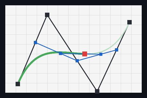
The animation draws the same construction for the current t. The dark
lines connect the control points, the blue lines and points are the
intermediate levels of interpolation, the red point is the result for this
t, and the green line is the curve traced so far. The small green
markers sit at t = 0, 0.1, 0.2, ..., 1. Edit the control points in the
code above and press "Compile & Run": three points give a quadratic curve,
four a cubic one, and more points a curve of higher degree.
What the construction tells you
A lot of a Bézier curve's behavior can be read directly from the construction, and checked numerically. For the curve in the sample:
- It starts at the first control point and ends at the last one. At
t = 0, every interpolation returns its left point, so the result isP0; att = 1, it is the last point. - It leaves the first point heading toward the second, and arrives at
the last point coming from the one before it. The direction at the
start matches the line from
P0toP1exactly, and likewise at the end. - It does not pass through the inner control points. For the sample
curve, it never gets closer than 182 pixels to
P1and 189 pixels toP2. They pull the curve toward them; they are not points on it. - It stays inside the convex hull of its control points, the smallest convex shape that contains all of them. Each interpolation produces a point between two points that already lie inside that hull, so the result can never leave it. Checked on 5,000 random curves with up to eight control points, not a single curve point fell outside.
Not evenly spaced
The green markers in the animation show something less obvious: equal
steps in t do not give equal distances along the curve. For the sample
curve, which is about 641 pixels long, the ten sections between the
markers range from 54 pixels in the middle to 92 pixels at the end. The
curve moves about 1.7 times as fast near its ends as in its middle.
For drawing that does not matter much, but anything that should move
along a curve at a constant speed, like an animation or text set along a
path, has to measure the curve's length and step through it by distance
instead of by t.
The formula behind it
Multiplying out all the interpolations gives a closed formula. For a
cubic curve with control points P0 to P3:
B(t) = (1-t)³·P0 + 3(1-t)²t·P1 + 3(1-t)t²·P2 + t³·P3
The weights in front of each point are the Bernstein polynomials, and for
any t they add up to 1, so B(t) is always a weighted average of the
control points, which is the convex hull property again. De Casteljau's
algorithm and this formula give the same curve: over 5,000 random curves
of degree 1 to 7, the two never differed by more than about 10⁻¹² pixels.
The formula is shorter to write down; the algorithm is easier to picture,
numerically very well-behaved, and works the same for any number of
points.
Why curves are usually cubic
With more control points, the curve becomes harder to steer. Every control point influences the entire curve, not just the part near it, and the curve follows the control polygon only loosely: try six points in the sample, and the result is a smooth arc that ignores most of the zigzag in between. That is why practical systems chain short, low-degree segments instead. TrueType fonts build their outlines from quadratic Bézier pieces, while PostScript and OpenType/CFF fonts, SVG paths, and most drawing programs use cubic ones, joined end to end, and wherever the outline should look smooth, each new segment starts in the direction the previous one ended.
Conclusion
A Bézier curve looks like a smooth, complicated shape, but de Casteljau's algorithm builds it from the simplest operation in geometry: finding a point partway along a straight line. Everything else, from where the curve starts and ends to why it stays within its control points, follows from repeating that one step.